Situation
Approximately 25% of the a product’s user-base (~42K) use the product, at least, once a month. However, given the nature of the service, where privacy is paramount, advertising revenue or selling user information aren’t a part of the business model. Optional support tiers are available for users to consider, but this business model has failed to sustain operations. There is recognition that a paid subscription or a Product + version is the only way to sustain and grow the business. An attempt at introducing a paid product has met with some success. It is assumed that usability of the product is linked to some of the financial outcomes.
Task
The client uses a combination of an off-the-shelf solution, along with Google Analytics, to monitor, communicate with, and understand their user base. There are over a 100 individual data points that are being tracked. Our job is to provide a non-partial recommendation on:
- How best to convert the current user base?
- Which existing features to include in a Freemium like offering?
- How best to structure, and link, data-driven research to product development (sustainable & repeatable revenue)?
- How best to expand the user base and expand operations?
- How best to communicate Data results with the client (interpret-ability is key)?
Action
After several conversations with the client it was decided to create an initial model of the current user base to understand which features were being used and if there was any link of usage to the existing business model.
Approach
A limit of 20 usability and financial outcome variables were selected (based on the initial conversations with the client) with the aim of performing logistic regression against the financial outcome of interest. A correlogram was created to assist in the visualization of data.
Corr-plot
After some data wrangling which involved the handling NAs and converting variables into factors the following corr-plot was observed.
- Understanding the corr-plot call
- scale while not strictly required for the cor() call, it is included here because we intend to use hierarchical clustering to order the grid.
- order = hclust Datacamp Tutorial on Heirarchical Clustering
- This was done to arrange the data using a clustering algorithm so that features used be grouped together to better understand user behavior.
- The remainder of the arguments are cosmetic - Link to package on cran
df_mini <- readRDS("article_data")
df_mini %>% scale() %>% cor() %>% corrplot(order = "hclust", hclust.method = "average",
                                            method = "color", diag = F,
                                            tl.col = "gray20",
                                            sig.level = T, addCoef.col = "white",
                                            number.cex = .6, type = "upper",
                                            tl.cex = 0.8)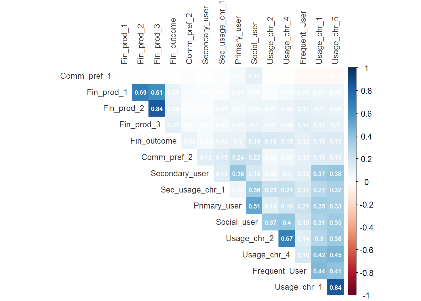
Interpretation of the corr-plot
- What does the corr-plot do?
- The corr-plot visualizes correlations between variables and provides a correlation co-efficient (optional) for each pair of potentially correlated variables.
- The dark blue color indicates high positive correlation, contrasted with the dark reds that indicate high negative correlation.
- Salient Features of this Corr-plot (Clustering)
- Financial Products 1, 2 and 3 cluster together
- Usage and Frequency of Usage characteristics cluster together
- However, there doesn’t seem to be an overlap between Financial Products and Usage.
- Salient Features of this Corr-plot (Correlation)
- Financial product 2 is highly correlated to Financial product 3.
- Buyer of one product likely buys the other.
- Usage Characteristic 1 is highly correlated to Usage Characteristic 5.
- Does one behavior lead to the other?
- Primary users are somewhat correlated to Social users (think some users have followers).
- Should followers be a paid feature?
- The correlations between Frequency users and User characteristics 1 and 5 should be explored.
- Who are the power users and what to they like doing? Note, from above Usage characteristics 1 & 5 are highly correlated.
- Financial Outcome is poorly correlated to Frequency and Usage.
- Financial product 2 is highly correlated to Financial product 3.
Logistic Regression
#Create a General Linear Model with glm()
Logistic_model <- glm(Fin_outcome ~ ., family = "binomial", data = df_mini)
summary(Logistic_model)
##
## Call:
## glm(formula = Fin_outcome ~ ., family = "binomial", data = df_mini)
##
## Deviance Residuals:
## Min 1Q Median 3Q Max
## -6.4655 -0.1647 -0.0753 -0.0624 3.5689
##
## Coefficients:
## Estimate Std. Error z value Pr(>|z|)
## (Intercept) -6.319e+00 1.855e-01 -34.071 < 2e-16 ***
## Primary_user -3.810e-03 4.071e-02 -0.094 0.925434
## Usage_chr_1 1.276e-05 6.538e-05 0.195 0.845266
## Usage_chr_2 1.907e-02 5.304e-03 3.596 0.000323 ***
## Sec_usage_chr_1 2.802e-03 1.688e-03 1.659 0.097074 .
## Frequent_User 9.427e-03 2.274e-03 4.145 3.40e-05 ***
## Social_user 1.268e-01 1.328e-02 9.545 < 2e-16 ***
## Comm_pref_1 -4.813e-02 1.308e-01 -0.368 0.712792
## Secondary_user -1.498e-03 1.878e-02 -0.080 0.936421
## Usage_chr_4 6.369e-04 1.533e-03 0.415 0.677809
## Usage_chr_5 1.294e-03 4.380e-04 2.955 0.003125 **
## Comm_pref_2 1.840e+00 1.600e-01 11.503 < 2e-16 ***
## Fin_prod_1 1.357e+00 3.013e-01 4.504 6.65e-06 ***
## Fin_prod_2 -1.400e-01 4.191e-02 -3.341 0.000835 ***
## Fin_prod_3 9.683e-02 2.648e-02 3.657 0.000256 ***
## ---
## Signif. codes: 0 '***' 0.001 '**' 0.01 '*' 0.05 '.' 0.1 ' ' 1
##
## (Dispersion parameter for binomial family taken to be 1)
##
## Null deviance: 4921.9 on 42359 degrees of freedom
## Residual deviance: 4159.2 on 42345 degrees of freedom
## AIC: 4189.2
##
## Number of Fisher Scoring iterations: 8Interpretation of Logistic Regression
The output of a logistic regression can be confusing because it describes the log-odds of something binary (yes/no) occurring. For example, a per unit increase in Usage Characteristic 2 increases the log odds of Financial Outcome by 1.097e-02. This doesn’t make sense to most people. However, we can transform log-odds into regular likelihood by calculating the exponential of the Estimate.
# Transform coefficients / Log - odds to interpret data
likelihood <- coef(Logistic_model) %>% exp() %>% round(2)
likelihood
## (Intercept) Primary_user Usage_chr_1 Usage_chr_2 Sec_usage_chr_1
## 0.00 1.00 1.00 1.02 1.00
## Frequent_User Social_user Comm_pref_1 Secondary_user Usage_chr_4
## 1.01 1.14 0.95 1.00 1.00
## Usage_chr_5 Comm_pref_2 Fin_prod_1 Fin_prod_2 Fin_prod_3
## 1.00 6.30 3.89 0.87 1.10Interpretation of Likelihood
- There is no increase or decrease in the likelihood of belonging to the class Financial Outcome based on whether the user is a Primary User or not.
- If a user has purchased Financial Product 1 then they are 3.89 times more likely to be a member of the Financial Outcome class as compared to a user who has not purchased Financial Product 1.
- Similarly, those that prefer Communication Methodology 2 are 6.3 times as likely to be a member of the class Financial Outcome.
Refining the Model
Removing insignificant variables using StepAIC()
trimmed_model <- stepAIC(Logistic_model, trace = 0)
trimmed_formula <- as.formula(summary(trimmed_model)$call)
trimmed_formula
## Fin_outcome ~ Usage_chr_2 + Sec_usage_chr_1 + Frequent_User +
## Social_user + Usage_chr_5 + Comm_pref_2 + Fin_prod_1 + Fin_prod_2 +
## Fin_prod_3New Model Likelihoods
New_model <- glm(trimmed_formula, family = "binomial", data = df_mini)
summary(New_model)
##
## Call:
## glm(formula = trimmed_formula, family = "binomial", data = df_mini)
##
## Deviance Residuals:
## Min 1Q Median 3Q Max
## -6.4141 -0.1646 -0.0757 -0.0626 3.5674
##
## Coefficients:
## Estimate Std. Error z value Pr(>|z|)
## (Intercept) -6.3615399 0.1501495 -42.368 < 2e-16 ***
## Usage_chr_2 0.0204807 0.0041681 4.914 8.94e-07 ***
## Sec_usage_chr_1 0.0027377 0.0016612 1.648 0.099349 .
## Frequent_User 0.0094607 0.0022414 4.221 2.43e-05 ***
## Social_user 0.1269422 0.0113836 11.151 < 2e-16 ***
## Usage_chr_5 0.0013975 0.0002659 5.255 1.48e-07 ***
## Comm_pref_2 1.8388259 0.1597747 11.509 < 2e-16 ***
## Fin_prod_1 1.3508331 0.3005187 4.495 6.96e-06 ***
## Fin_prod_2 -0.1400212 0.0419752 -3.336 0.000851 ***
## Fin_prod_3 0.0972642 0.0264823 3.673 0.000240 ***
## ---
## Signif. codes: 0 '***' 0.001 '**' 0.01 '*' 0.05 '.' 0.1 ' ' 1
##
## (Dispersion parameter for binomial family taken to be 1)
##
## Null deviance: 4921.9 on 42359 degrees of freedom
## Residual deviance: 4159.7 on 42350 degrees of freedom
## AIC: 4179.7
##
## Number of Fisher Scoring iterations: 8likelihood_new <- coef(New_model) %>% exp() %>% round(2)
likelihood_new## (Intercept) Usage_chr_2 Sec_usage_chr_1 Frequent_User Social_user
## 0.00 1.02 1.00 1.01 1.14
## Usage_chr_5 Comm_pref_2 Fin_prod_1 Fin_prod_2 Fin_prod_3
## 1.00 6.29 3.86 0.87 1.10R2 - Goodness of Fit - Equivalents for Logistic regression
LogRegR2(New_model)## Chi2 762.1696
## Df 9
## Sig. 0
## Cox and Snell Index 0.01783177
## Nagelkerke Index 0.1625578
## McFadden's R2 0.1548541Interpretation of the Goodness of Fit
Generally a fit below 0.2 is considered poor. In other words, while the model may be significant as indicated by the p-values, the explanation of variation in the underlying model is not good enough.
Additional refinement of the model
It was decided to create a model of only those users that preferred Communication Preference 2. It was recognized that focusing on these users would, effectively, half the target audience, however, focusing on a narrower but potentially predictable audience was considered an acceptable trade-off.
summary(New_model_2)##
## Call:
## glm(formula = trimmed_formula_2, family = "binomial", data = df_mini_2)
##
## Deviance Residuals:
## Min 1Q Median 3Q Max
## -6.8272 -0.1754 -0.1631 -0.1521 3.0355
##
## Coefficients:
## Estimate Std. Error z value Pr(>|z|)
## (Intercept) -4.597231 0.070415 -65.288 < 2e-16 ***
## Usage_chr_2 0.024043 0.004360 5.515 3.49e-08 ***
## Sec_usage_chr_1 0.002736 0.001675 1.633 0.10238
## Frequent_User 0.008813 0.002250 3.917 8.95e-05 ***
## Social_user 0.143481 0.011855 12.103 < 2e-16 ***
## Usage_chr_5 0.001511 0.000268 5.639 1.71e-08 ***
## Fin_prod_1 1.390755 0.300556 4.627 3.71e-06 ***
## Fin_prod_2 -0.133313 0.041833 -3.187 0.00144 **
## Fin_prod_3 0.087803 0.026078 3.367 0.00076 ***
## ---
## Signif. codes: 0 '***' 0.001 '**' 0.01 '*' 0.05 '.' 0.1 ' ' 1
##
## (Dispersion parameter for binomial family taken to be 1)
##
## Null deviance: 3920.8 on 20774 degrees of freedom
## Residual deviance: 3451.8 on 20766 degrees of freedom
## AIC: 3469.8
##
## Number of Fisher Scoring iterations: 7New Likelihood of only those who chose Communication Preference 2
coef(New_model_2) %>% exp() %>% round(2)## (Intercept) Usage_chr_2 Sec_usage_chr_1 Frequent_User Social_user
## 0.01 1.02 1.00 1.01 1.15
## Usage_chr_5 Fin_prod_1 Fin_prod_2 Fin_prod_3
## 1.00 4.02 0.88 1.09Refined Goodness of Fit
LogRegR2(New_model_2)## Chi2 468.9662
## Df 8
## Sig. 0
## Cox and Snell Index 0.0223207
## Nagelkerke Index 0.1297812
## McFadden's R2 0.1196099Even more refinement?
## How many users engage in Financial Product 1?## # A tibble: 1 x 1
## n
## <int>
## 1 97There aren’t enough users to make a business case.
Result
To re-cap, we’ve performed three methods of data - analysis, which I’ll argue are being used as exploratory methods.
The hierarchical clustering resulted in a some-what neat division of users who self-aggregated into:
- Those that use / purchase Financial products 1, 2, and 3.
- Those that behave in the manner as described by Usage Characteristics 1 and 5
- Those that behave in the manner of Usage Characteristics 2 and 4
- A small cluster around Primary and Secondary users.
- Finally, there doesn’t seem to be any clustering around Financial Outcome.
The correlogram supports the interest in the clustering of Financial Products, and Usage Characteristics 1 and 5, along with the apparent randomness of Financial Outcome.
Finally, the logistic regression suggests that the likelihood of Financial Outcome could be based on the presence or absence of behaviors associated with Financial Product 1 and Communication Preference 2.
However, the goodness of fit indices for the model of all users indicated that it wasn’t a very good model.
To improve the model it was decided to focus on those users who preferred Communication Preference 2, however, after creating and trimming the new logistic model, the goodness of fit indices still indicated that the model didn’t do a good job of explaining why users engaged in Financial Outcome.
Further refinement of the model was not considered because the cohort of users engaged with Financial Product 1 was deemed too small.
The final conclusion reached was that the Financial Outcome of interest occurred in a way that currently captured variables were not able to model.
Talk (with the Client)
We went back and presented our results. After some discussion. The Product Owners believed that a combination of certain Usability Behaviors (being measured) in conjunction with a Value Proposition 1 (not being measured) was key to Financial Outcome.
SMART Goals
A/B Test Communication Preference 2 and Communication Preference 2 with respect to establishing a cohort of those that agree with Value Proposition 1
Seek Financial Outcome behavior and compare cohorts of those that agree and disagree with Value Proposition 1 as a means to create a baseline for future product iterations.
Learnings
- In typical MBA fashion, I’m calling this process STAR - T - SMART.
- Product Owners / Start-up Founders have a strong sense of, qualitatively, why users engage in behavior. It is important to get them to articulate their intuition in a way that can be quantitatively measured.
- Quantitative measures of Behavior or Value Propositions need to link to Financial Outcomes = Business Models.