Overview
The Central Limit Theorem (CLT) states that the sampling distribution of the mean (average of many sample means) will approximate a normal distribution as the sample size - or number of samples - increases, regardless of the nature of the population distribution from which the samples are obtained, as long as the samples are \(iid\)1. While an individual sample has a mean and variance, the average of many means, of such samples, has its own variance (\(VAR = \sigma^2 / n\)) centered around the population mean and its own standard deviation (\(SD = \sigma / \sqrt{n}\)), where \(n\) is the sample size. Per definition, the sampling distribution of the mean is an unbiased estimator of the population average.
Simulations
For the purposes of the assignment the population being sampled follows an exponential distribution2 with the rate \(\lambda = 0.2\). Both the \(Mean\) and \(SD\) of this distribution \(= {1}/\lambda = 5\), hence \(VAR = {1}/\lambda^2 = 25\). The following code generates a single sample from the exponential population using the rexp(n, rate = ) function, with the desired length of the sample \(n=40\), and the rate (\(lambda\)) = 0.2.
set.seed(45)
sample1 <- rexp(40, rate = 0.2)
To demonstrate the CLT, we will take 1000 samples of \(n = 40\) from the population, compute the sampling distribution of the mean, and compare the sampling distribution statistic to those we expect, given the population characteristics. The following code borrowed from the motivating example in the submission instructions creates an empty vector mns and then loops over the expression mean(rexp(40, rate = 0.2)) to create a vector of length 1000 by concatenating each sample average.
mns = NULL
for (i in 1 : 1000) mns = c(mns, mean(rexp(40, rate = 0.2)))
Sample Mean V. Theorectical Mean V. Sampling Distribution of the Mean
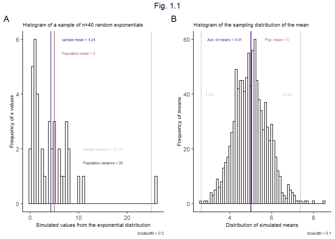
Figure 1.1.A shows a histogram of one sample (\(n = 40\)) from an exponential distribution with \(\lambda = 0.2\). The average of this sample is 4.24. Note the difference between the sample mean (in blue) and the known population mean (in red). The mean for a single sample is governed by the variability of that sample, simulated here at random.
Figure 1.1.B shows a histogram of the sampling distribution of the mean (1000 samples, each of size \(n = 40\)). Per theory, the average of these averages 5.01 is a better estimator of the population average because of the Law of Large Numbers (LLM)3
Sample Variance V. Theorectical Variance V. Standard Error of the Mean
The sample variation is calculated by \(\frac{\sum({x_i} - \bar{x})^2} {n - 1}\) where \(x_i\) is the sample vector, \(\bar{x}\) is the sample average, and \(n\) is the sample size. The expected variance of the population is given by \({1} / \lambda^2\) = 25. The variance of the sampling distribution of the mean, however, is the variation among the averages of each sample and is centered around the population mean. We expect \(VAR = \sigma^2 / n\) i.e. \(\frac{({1}/\lambda)^2}{40}\) = \(\frac{({1}/{0.2})^2}{40}\) = 0.625. Compare this value to the actual variance 0.65 of the simulated sample of 1000 exponentials.
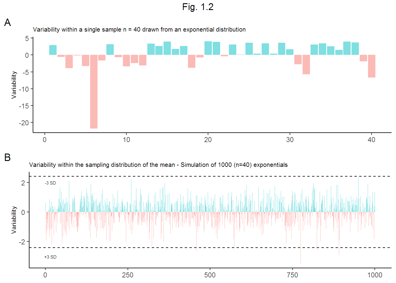
Figure 1.2(A) shows the difference between the variation within a sample and the theoretical variance of the population. Figure 1.2(B) shows the variation among the average of 1000 \(n=40\) samples. Note that there is less variation among the sample means.
Is the Sampling Distribution of the Mean Normal?
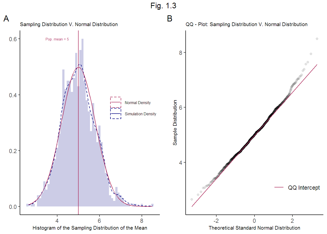
Figure 1.3.A shows a normal density plot (mean = 5, SD = 0.8 mirroring the sampling distribution) superimposed over density plot of the sampling distribution of the mean. Fig. 1.3.B is a QQ-plot comparing the quantiles of a standard normal density to the sampling distribution density. Note the similarity in the density distributions in subplot A. The tails of the sampling distribution deviate slightly from the tails of the standard normal in subplot B. While this is to be expected beyond the 2-SD zone, per theory, a simulation with a larger sample size would be even closer to standard normal.
The little deviation between the two distributions demonstrates that the sampling distribution of the mean is nearly normal.
If the population variation is unknown, we can substitute the population \(\sigma\) with sample standard deviation \(s\) to calculate what is referred to as the standard error of the mean (how variable the sample averages are) i.e. \(SE = s / \sqrt{n}\).
This equation is one of the building blocks of statistical inference, because we now know how unlikely deviations from the expected population average might be, based on the properties of the normal distribution, reflected by the Z score4 or a T-statistic5.
Appendix
This report provides a brief overview of the Central Limit Theorem for the purposes of fulfilling the submission requirements for the Statistical Inference course offered by Johns Hopkins University’s Bloomberg School of Public Health on Coursera - link.
Code for this report can be found on Github.